The gamma distribution is widely used in climatological applications for representing variations in precipitation, ranging from seasonal and monthly totals (e.g., Ropelewski et al. 1985, Waggoner 1989) to nonzero daily values (e.g., Stern and Coe 1984, Wilks 1989). In addition, it can be used to interpret the 30- and 90-day precipitation forecasts issued by the Climate Analysis Center (Wilks and Eggleston 1992).
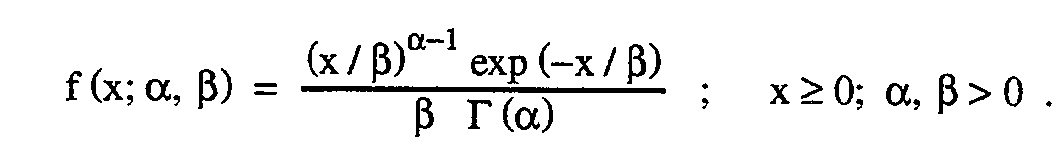
The probability density function for this distribution can be written as
Here x is the random variable (e.g., the precipitation amount), α and β are the two distribution parameters, and Γ denotes the gamma function. The gamma distribution is characterized by mean µ=αβ and variance σ^2=αβ^2.
The scale parameter β serves, as its name implies, only to scale the distribution. This can be appreciated by noting that everywhere the random variable x appears in the probability density it is divided by β. Since the scale parameter carries the dimensional information, it is sometimes useful to work with the "standard" gamma distribution, i.e., with β = 1.
Gamma distribution probabilities are calculated by integrating the probability density function. In particular, cumulative probability, i.e., the probability that the random variable x will be on larger than a specific value, r, is given by

This integration cannot be performed analytically, and numerical methods are required to evaluate the integral. Extensive results of such integrations are tabulated in this publication. The probability that the random variable x will fall within any interval can be obtained by finding the difference between the cumulative probabilities:

24 pp.